Gossip Averaging
Gossip averaging is an important component in consensus-based decentralized learning algorithms. Gossip-based computation can be used to compute random samples, quantiles, or any other aggregate-based queries in a decentralized manner. In this post, we will look into the gossip-averaging algorithm which aims to compute the average of the given decentralized system with fixed graph topology in linear time. In the decentralized setup, every node only communicates with its neighbors and the time (hops) required to pass the information from node $i$ to $j$ is equal to the shortest path length from $i$ to $j$.
Note that there are many ways to implement distributed averaging. One straightforward method is flooding. In this method, each node maintains a table of the initial values of all the nodes, initialized with its own node value. At each iteration, the nodes exchange the non-trivial information from their own tables with their neighbors. After a number of iterations equal to the diameter of the network, every node knows all the initial values of all the nodes, so the average can be computed. However, the flooding algorithm has a memory overhead proportional to the number of nodes in the system. Gossip averaging gets rid of this memory overhead.
Notations:
- Goal: Compute the average of initial values in an $n$-node decentralized system.
- Connectivity: Sparse graph topology G(N,E). N = set of nodes = { $1,…,n$ }. E = set of edges.
- Adjacency/Mixing Matrix (W): $0 \leq w_{ij} < 1$ and $w_{ij} \neq 0$ for { $i,j$ } $\in E$.
- Neighbors of node-$i$: $N_i$ represents all $j$’s such that $w_{ij} \neq 0$.
- Initial values: $x_i^{(0)}$ $\forall i \in [1,…,n]$
Gossip Averaging Algorithm:
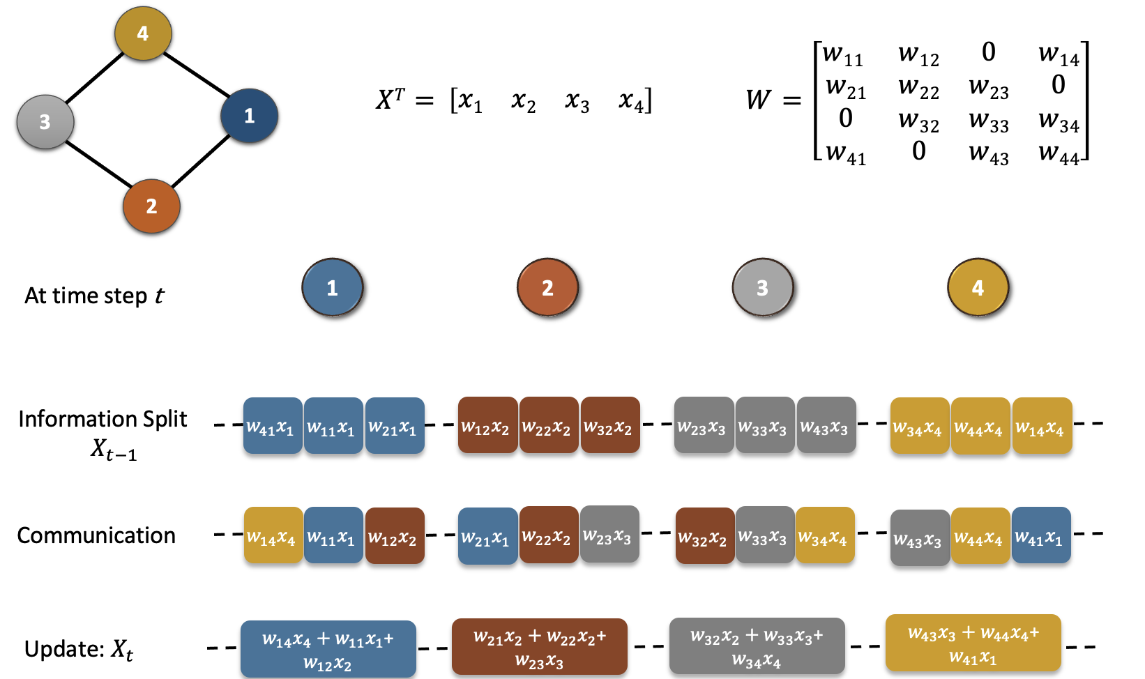
At every iteration of gossip averaging, there are three steps (refer to Figure 1):
- Information Split: Each node first splits the information based on corresponding column weights of W.
- Communication: Communicates the split information to respective neighbors.
- Aggregation: Each node updates its value by adding the received information.
In summary, the matrix representation of one iteration of gossip averaging is given by $X_t = W X_{t-1}$. Unrolling the recursion: $X_t = W^t X_0$.
where $X_t^T = [x_1^t, x_2^t,…,x_n^t]$ and $x_i^t$ is the data/value on $i^{th}$ node at iteration $t$.
Convergence:
The gossip averaging algorithm converges in linear time with respect to the number of nodes i.e., $O(n)$. The following are the constraints required for the linear convergence of the gossip averaging algorithm.
- Strongly Connected Graph: There is a path from each node to every other node.
- Self Loops: Each node is connected to itself.
- Doubly Stochastic Mixing Matrix: This implies two conditions
- Column stochasticity: Each column sums to one. This ensures that the average of the system is preserved at each iteration.
- Row stochasticity: Each row sums to one. This ensures that the addition of received information results in a valid weighted averaging.
- Symmetric Mixing Matrix: This property helps in the convergence analysis and makes the practical realization of doubly stochastic mixing possible.
These constraints require the graph to be undirected and static. However, the PushSum variant of the algorithm which communicates weights along with data allows the graph to be directed and time-varying.
Properties of Doubly Stochastic Matrices:
Let $W \in [0, 1]^{n \times n}$ be a doubly stochastic matrix and $\mathbf{1}$ be a column matrix with every element as 1.
- Row stochasticity: $W \mathbf{1}$ = $\mathbf{1}$
- Column stochasticity: $\mathbf{1}^T$ $W$ = $\mathbf{1}^T$
- The largest eigenvalue of $W$ is 1 i.e., $\lambda_1(W)=1$
- The absolute eigenvalue of $W$ is bounded by 1 i.e., $| \lambda_i(W) | \leq 1$ $\forall i \in [1,n]$
Spectral Gap:
The spectral gap ($\rho$) of a doubly stochastic matrix is defined as $| \lambda_2(W) |$ where $1= | \lambda_1(W) | > | \lambda_2(W) | \geq … \geq | \lambda_n(W) |$ are the ordered eigenvalues of $W$.
$\therefore \rho = | \lambda_2(W) | \in [0, 1)$
A smaller spectral gap indicates that the graph has more connectivity and vice versa. In particular, a fully connected graph with uniform weights has zero spectral gap i.e., $\rho = | \lambda_2(W) | = 0$. The spectral gap (defined as $\delta = 1 - \rho$) for different topologies can be found in Table 1 of the CHOCO-SGD paper. Note that some papers also define $(1-| \lambda_2(W) |)$ or $| \lambda_2(W) |^2$ as spectral gap. However, we will consider the second-largest absolute eigenvalue of $W$ as the spectral gap of the connectivity graph.